Population Initialization, Squashing, and Snapshot Management in LASER

Note

EULA = Epidemiologically Uninteresting Light Agent

An EULA is an agent that no longer affects disease dynamics (e.g., permanently recovered or immune individuals) and can be compressed into aggregate counts rather than tracked individually.

As the number agents in your LASER population model grows (e.g., 1e8), it can become computationally expensive and unnecessary to repeatedly run the same (sophisticated) initialization routine every sim. In many cases -— particularly during model calibration -— it is far more efficient to initialize the population once, save it, and then reload the initialized state for subsequent runs.

This approach is especially useful when working with EULAs – Epidemiologically Uninteresting Light Agents. For example it can be a very powerful optimization to compress all the agents who are already (permanently) recovered or immune in a measles or polio model into a number/bucket. In such models, the majority of the initial population may be in the “Recovered” state, potentially comprising 90% or more of all agents. If you are simulating 100 million agents, storing all of them can result in punitive memory usage.

To address this, LASER supports a squashing process. Squashing involves defragmenting the data frame such that all epidemiologically active or “interesting” agents (e.g., Susceptible or Infectious) are compacted to the beginning of the array. After squashing, only array indices [0:count] contain valid data. The remaining memory region [count:capacity] is no longer considered valid and will be overwritten when new agents are added (e.g., through births).

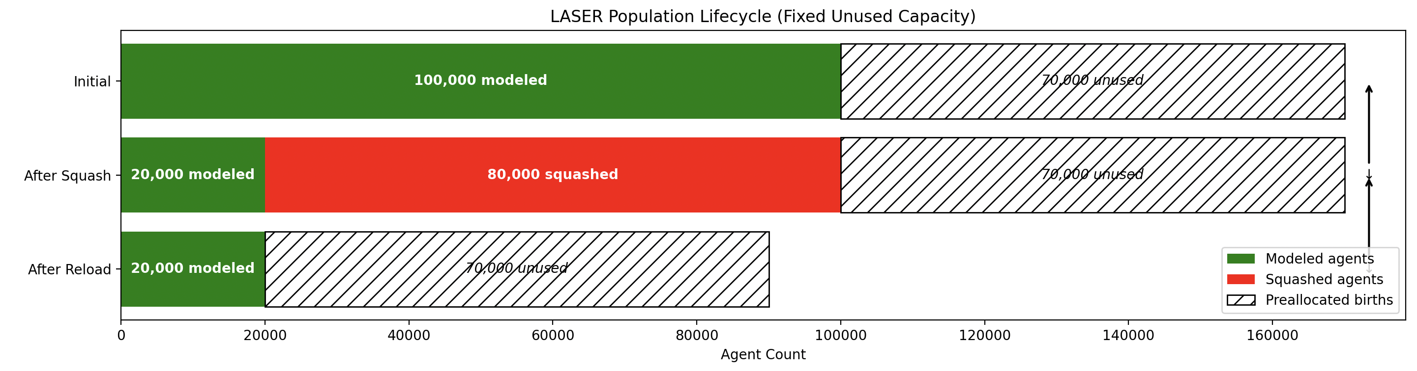
Memory layout of LASER population arrays. Active (modeled) agents occupy indices [0:count], squashed agents exist in the region [count:capacity] until save/load, and future capacity reserves space for unborn agents (e.g., births). Saving and reloading acts as a defragmentation operation, reclaiming the squashed region.

Some notes about squashing:

• The population count is adjusted so that all for loops and step functions iterate only over the active population.

• This not only reduces memory usage but also improves performance by avoiding unnecessary computation over inactive agents.

Some caveats about using saved populations: - You will want to be confident that the saved population is sufficiently randomized and representative; - If you are calibrating parameters used to create the initial population in the first place, you’ll need to recreate those parts of the population after loading, diminishing the benefit of the save/load approach.

When saving a Snapshot, note that only the active (unsquashed) portion of the population is saved. Upon reloading:

• Only this subset is allocated in memory.

• This prevents the performance penalty of managing large volumes of unused agent data.

Important Detail

Before squashing, you should count and record the number of recovered (or otherwise squashed) agents. This count should be stored in a summary variable —- typically the R column of the results data frame. This ensures your model retains a complete epidemiological record even though the agents themselves are no longer instantiated.

Implementation Details: How to Add Squashing, Saving, Loading, and Correct R Tracking to a LASER SIR Model

1. Add Squashing

• Add a `squash_recovered()` function This should call LaserFrame.squash(…) with a boolean mask that includes non-recovered agents (disease_state != 2). You may choose a different criterion, such as age-based squashing.

• Count your “squashed away” agents first You must compute and store all statistics related to agents being squashed before the squash() call. After squashing, only the left-hand portion of the arrays (up to .count) remains valid.

• Seed infections timing depends on your workflow

  • If squashing then running immediately: Seed infections after squashing. Otherwise, infected agents may be inadvertently removed.

  • If squashing then saving for later: Seed infections before squashing so they are included in the saved snapshot.

• Store the squashed-away totals by node Before squashing, compute and record node-wise totals (e.g., recovered counts) in results.R[0, :] so this pre-squash information persists.

• Optionally simulate EULA effects once and save If modeling aging or death among squashed agents, simulate this up front and store the full [time, node] matrix (e.g., results.R[:, :]). This avoids recomputation at runtime.

2. Save Function

Implement a save(path) method:

• Use LaserFrame.save_snapshot(path, results_r=..., pars=...)

• Include:

  • The post-squash active population (only array indices [0:count] are saved; squashed agents are not included)

  • The results.R matrix containing both pre-squash and live simulation values

  • The full parameter set in a PropertySet

3. Load Function

Implement a load(path) class method:

• Call LaserFrame.load_snapshot(path, cbr, nt) to retrieve:

  • Population frame (with capacity automatically calculated based on expected births)

  • Results matrix

  • Parameters

• The cbr (crude birth rate per 1000/year) and nt (simulation duration in ticks) parameters are required if your model includes births. LASER will automatically calculate the appropriate capacity to accommodate population growth. If not modeling births, pass cbr=None and nt=None to set capacity = count.

• Reconstruct all components using init_from_file()

Warning

Vital Dynamics Considerations

When modeling vital dynamics—especially births—there is an additional step to ensure consistency after loading:

• Property initialization for unborn individuals must be repeated if your model pre-assigns properties up to .capacity. For example, if timers or demographic attributes (like date_of_birth) are pre-initialized at t=0, you must ensure this initialization is re-applied after loading, because only the .count population is reloaded, not the future .capacity.

Failing to do so may result in improperly initialized agents being birthed after the snapshot load, which can lead to subtle or catastrophic model errors.

4. Preserve EULA’d Results

• Use ``+=`` to track new recoveries alongside pre-squash R values In run(), use additive updates so that pre-saved recovered agents are preserved:

  self.results.R[t, nid] += ((self.population.node_id == nid) &
                             (self.population.disease_state == 2)).sum()
  

  This works because results.R was pre-populated with squashed agent counts before squashing (see step 1 above, where populate_results() records node-wise recovered totals). The += operator adds new recoveries during the simulation to these pre-existing counts, ensuring your output accounts for both squashed-away immunity and recoveries during the live simulation.

Complete SIR LASER Model with Squashing and Snapshot Support

This example demonstrates a complete SIR model using LASER, featuring:

• Agent squashing based on recovery state

• Pre-squash result capture

• Snapshot saving and loading

• Node-level time series tracking

• Plotting of total S, I, and R dynamics

import numpy as np
import click
import matplotlib.pyplot as plt
from pathlib import Path

from laser.core import LaserFrame, PropertySet

class Transmission:
    """
    A simple transmission component that spreads infection within each node.
    """
    def __init__(self, population, pars):
        self.population = population
        self.pars = pars

    def step(self):
        """
        For each node in the population, calculate the number of new infections as a function of:
        - the number of infected individuals,
        - the number of susceptibles,
        - adjustments for migration and seasonality,
        - and individual-level heterogeneity.

        Then, select new infections at random from among the susceptible individuals in each node,
        and initiate infection in those individuals.
        """
        pass  # Implementation omitted for documentation purposes

    @classmethod
    def init_from_file(cls, population, pars):
        return cls(population, pars)

class Progression:
    """
    A simple progression component that recovers infected individuals probabilistically.
    """
    def __init__(self, population, pars):
        self.population = population
        self.pars = pars

    def step(self):
        """
        At each time step, update the disease state of infected individuals based on the model's
        progression logic. This may be driven by probabilities, timers, or other intrahost dynamics.
        """
        pass  # Implementation omitted for documentation

    @classmethod
    def init_from_file(cls, population, pars):
        return cls(population, pars)

class RecoveredSquashModel:
    """
    A simple multi-node SIR model demonstrating use of LASER's squash and snapshot mechanisms.
    """
    def __init__(self, num_agents=100000, num_nodes=20, timesteps=365):
        self.num_agents = num_agents
        self.num_nodes = num_nodes
        self.timesteps = timesteps
        self.population = LaserFrame(capacity=num_agents, initial_count=num_agents)
        self.population.add_scalar_property("node_id", dtype=np.int32)
        self.population.add_scalar_property("disease_state", dtype=np.int8)  # 0=S, 1=I, 2=R

        self.results = LaserFrame(capacity=self.num_nodes)
        self.results.add_vector_property("S", length=timesteps, dtype=np.int32)
        self.results.add_vector_property("I", length=timesteps, dtype=np.int32)
        self.results.add_vector_property("R", length=timesteps, dtype=np.int32)

        self.pars = PropertySet({
            "r0": 2.5,
            "migration_k": 0.1,
            "seasonal_factor": 0.8,
            "transmission_prob": 0.2,
            "recovery_days": 14
        })

        self.components = [
            Transmission(self.population, self.pars),
            Progression(self.population, self.pars)
            # could add other components like vaccination
        ]

    def initialize(self):
        np.random.seed(42)
        self.population.node_id[:] = np.random.randint(0, self.num_nodes, size=self.num_agents)
        recovered = np.random.rand(self.num_agents) < 0.6
        self.population.disease_state[:] = np.where(recovered, 2, 0)

    def seed_infections(self):
        susceptible = self.population.disease_state == 0
        num_seed = max(1, int(0.001 * self.population.count))
        seed_indices = np.random.choice(np.where(susceptible)[0], size=num_seed, replace=False)
        self.population.disease_state[seed_indices] = 1

    def squash_recovered(self):
        """
        Removes all agents who are recovered (state 2).
        This reduces memory footprint and speeds up simulation.
        """
        keep = self.population.disease_state[:self.population.count] != 2
        self.population.squash(keep)

    def populate_results(self):
        """
        Populate initial R values before squashing to reflect the pre-squash immunity landscape.
        """
        for nid in range(self.num_nodes):
            initial_r = ((self.population.disease_state == 2) & (self.population.node_id == nid)).sum()
            decay = np.linspace(initial_r, initial_r * 0.9, self.timesteps, dtype=int)
            self.results.R[:, nid] = decay
        print("Initial R counts per node:", self.results.R[0, :])
        print("Total initial R (summed):", self.results.R[0, :].sum())

    def run(self):
        for t in range(self.timesteps):
            for component in self.components:
                component.step()
            for nid in range(self.num_nodes):
                self.results.S[t, nid] = ((self.population.node_id == nid) & (self.population.disease_state == 0)).sum()
                self.results.I[t, nid] = ((self.population.node_id == nid) & (self.population.disease_state == 1)).sum()
                self.results.R[t, nid] += ((self.population.node_id == nid) & (self.population.disease_state == 2)).sum()

    def save(self, path):
        """
        Save the current model state to an HDF5 file, including population frame,
        pre-squash results, and simulation parameters.
        """
        self.population.save_snapshot(path, results_r=self.results.R, pars=self.pars)

    @classmethod
    def load(cls, path, cbr=35.0, sim_duration=365):
        """
        Reload a model from an HDF5 snapshot. Note: reloaded population will have
        only post-squash agents (e.g., susceptibles and infected).

        Args:
            path: Path to the snapshot HDF5 file
            cbr: Crude birth rate (per 1000/year) for capacity calculation
            sim_duration: Simulation duration in days for capacity calculation
        """
        pop, results_r, pars = LaserFrame.load_snapshot(path, cbr=cbr, nt=sim_duration)
        model = cls(num_agents=pop.capacity, num_nodes=results_r.shape[1], timesteps=results_r.shape[0])
        model.population = pop
        model.results.R[:, :] = results_r
        model.pars = PropertySet(pars)
        model.components = [
            Transmission.init_from_file(model.population, model.pars),
            Progression.init_from_file(model.population, model.pars)
        ]
        return model

    def plot(self):
        """
        Plot the time series of total S, I, and R across all nodes.
        """
        # details omitted

@click.command()
@click.option("--init-pop-file", type=click.Path(), default=None, help="Path to snapshot to resume from.")
@click.option("--output", type=click.Path(), default="model_output.h5")
def main(init_pop_file, output):
    if init_pop_file:
        model = RecoveredSquashModel.load(init_pop_file)
        model.run()
        model.plot()
    else:
        model = RecoveredSquashModel()
        model.initialize()
        model.seed_infections()
        model.populate_results()
        model.squash_recovered()
        model.save(output)
        print(f"Initial population saved to {output}")

if __name__ == "__main__":
    main()